In this notebook we’ll perform a rudimentary genome-wide association study using the 1000 Genomes (1KG) dataset. The goal of this tutorial is to demonstrate the mechanics of performing genome-wide analyses using variant call data stored with TileDB-VCF and how such analyses can be easily scaled using TileDB’s serverless computation platform.
To get started we’ll load a few required packages and define several variables that we’ll refer to throughout the notebook.
Setup
Packages
import tiledbimport tiledbvcfimport tiledb.cloudfrom tiledb.cloud.compute import Delayedimport numpy as npimport seaborn as snsimport matplotlib as mplimport matplotlib.pyplot as pltprint(f"tileDB-vcf v{tiledbvcf.version}\n"f"tileDB-cloud v{tiledb.cloud.version.version}")
!tiledbvcf stat --uri tiledb://TileDB-Inc/vcf-1kg-phase3
/bin/bash: line 1: tiledbvcf: command not found
Sample Phenotypes
Because no phenotypic data was collected for the 1KG dataset, we’ll create a dummy trait indicating whether or not a sample identified as female.
with tiledb.open(sample_array) as A: df_samples = A.df[:]# dummy traitdf_samples["is_female"] = df_samples.gender =="female"df_samples
pop
super_pop
gender
is_female
sampleuid
HG00096
GBR
EUR
male
False
HG00097
GBR
EUR
female
True
HG00099
GBR
EUR
female
True
HG00100
GBR
EUR
female
True
HG00101
GBR
EUR
male
False
...
...
...
...
...
NA21137
GIH
SAS
female
True
NA21141
GIH
SAS
female
True
NA21142
GIH
SAS
female
True
NA21143
GIH
SAS
female
True
NA21144
GIH
SAS
female
True
2504 rows × 4 columns
Scaling GWAS with Serverless UDFs
We can parallelize the association analysis by dividing the genome into disjoint partitions that are queried, filtered, and analyzed by separate serverless nodes.
Binned Genomic Regions
To get started we’ll use the genome_windows UDF to divide a genome into windows (i.e., bins) and return a list of regions in the chr:start-end format that tiledbvcf expects.
Each of the individual tasks we performed above must be wrapped in functions so they can be packaged as UDFs and shipped to the serverless compute infrastructure. We’ll define two separate functions:
1. vcf_snp_query()
queries a specified window from the genome
filters the sites based on the defined criteria
%%timeres = tiledb.cloud.udf.exec( func ="aaronwolen/vcf_snp_query", uri = array_uri, attrs = attrs, regions = bed_regions[:2],)res.to_pandas()
CPU times: user 94.3 ms, sys: 62.6 ms, total: 157 ms
Wall time: 9.48 s
CPU times: user 90.5 ms, sys: 23 ms, total: 113 ms
Wall time: 9.66 s
contig
pos_start
oddsratio
pvalue
0
20
61098
0.494083
0.482112
1
20
61138
0.289018
0.590851
2
20
61795
0.068686
0.793260
3
20
63231
0.851720
0.356066
4
20
63244
0.004420
0.946994
...
...
...
...
...
423
20
198965
0.150694
0.697873
424
20
198977
0.025577
0.872937
425
20
199078
0.000250
0.987379
426
20
199114
0.000250
0.987379
427
20
199986
0.000250
0.987379
428 rows × 4 columns
4. combine_results()
creates a single dataframe containing individual results from each partition
def combine_results(dfs):""" Combine GWAS Results :param list of dataframes: Region-specific GWAS results to combine """import pyarrow as paprint(f"Input list contains {len(dfs)} Arrow tables") out = pa.concat_tables([x for x in dfs if x isnotNone])return out
Construct UDF-based Task Graph
To run the complete pipeline serverlessly we need to create Delayed versions of these functions with the appropriate parameters. For query_region() we need to create one delayed instance for each of the genomic regions to be queried in parallel.
nregions =len(bed_regions[:100])nparts = nregions //5print(f"Analyzing {nregions} regions across {nparts} partitions")delayed_queries = []for i inrange(nparts): delayed_queries.append( Delayed("aaronwolen/vcf_snp_query", result_format=tiledb.cloud.UDFResultType.ARROW, name=f"VCF SNP Query {i}", )( uri=array_uri, attrs=attrs, regions=bed_regions[:nregions], region_partition=(i, nparts), memory_budget_mb=1024, ) )delayed_filters = [ Delayed("aaronwolen/filter_variants", name=f"VCF Filter {i[0]}")( df=i[1], maf=(0.05, 0.95) )for i inenumerate(delayed_queries)]delayed_gwas = [ Delayed("aaronwolen/calc_gwas", name=f"VCF GWAS {i[0]}")( df=i[1], trait=df_samples.is_female )for i inenumerate(delayed_filters)]delayed_results = Delayed(combine_results, local=True)(delayed_gwas)delayed_results.visualize()
Analyzing 100 regions across 20 partitions
Finally, we can execute our distributed GWAS and collect the results.
Input list contains 20 Arrow tables
CPU times: user 18.4 s, sys: 11.7 s, total: 30.1 s
Wall time: 3min 11s
results.to_pandas()
contig
pos_start
oddsratio
pvalue
0
20
61098
0.494083
0.482112
1
20
61138
0.289018
0.590851
2
20
61795
0.068686
0.793260
3
20
63231
0.851720
0.356066
4
20
63244
0.004420
0.946994
...
...
...
...
...
30836
20
9999302
1.173945
0.278592
30837
20
9999622
1.173945
0.278592
30838
20
9999661
1.173945
0.278592
30839
20
9999900
0.999755
0.317370
30840
20
9999996
0.261170
0.609317
30841 rows × 4 columns
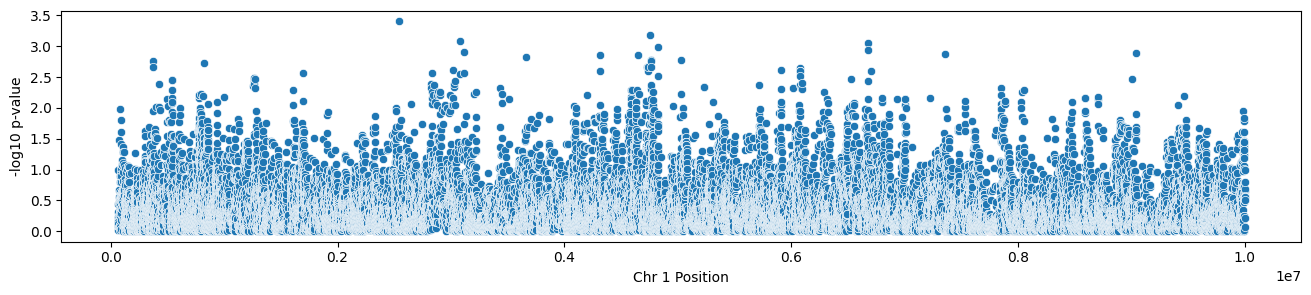
And no association test would be complete without a manhattan plot:
results = results.to_pandas()results["log_pvalue"] =-np.log10(results.pvalue)plt.figure(figsize = (16, 3))ax = sns.scatterplot( x ="pos_start", y ="log_pvalue", data = results)ax.set(xlabel ="Chr 1 Position", ylabel ="-log10 p-value")
Summary
Here we’ve demonstrated how genome-wide pipelines can be encapsulated as distinct tasks, distributed as UDFs, and easily deployed in parallel at scale.